A very simple discrete algorithm for smoothing out impulses to a target constant value

Demand smoothing

Let’s assume you use a lot of toilet paper at your home. Some number of rolls per week(integer rolls). If you buy new packages of toilet paper once a month, let’s figure out a simple algorithm to keep your bathroom well-stocked.

Roll up weekly data

Each week, we have our usage, but since we’re only buying once every month we need to consider the sum over the weeks inside. Consider M-S weeks, then the months have the following number of Sundays:

[4,4,4,5,4,4,5,4,5,4,4,5]

We’ll return to this later.

Available rolls

We dont want to run out, period. As not-a-risk taker, and someone who occasionally throws parties, I want at least twice as much TP around as I normally need. Let’s then say whatever my biggest usage per week is, times two, will be my target t.

Minimizing Error

Because we have a target for available rolls, our goal throughout the month, is to have our order keep us as close to that value as possible.

For i, \(1 ≤ i ≤ 5\) the numbered weeks in the month, and u_i the corresponding TP usages. Also assume that before you buy some more TP, you have o the “on shelf” TP from the month before. We’ll be calculating our TP purchase x

We wish to minimize

\[\mathop{\arg\,\min}\limits_x\left(\sum_i\left(\mid x+o-\sum^i_j u_j -t \mid\right)\right)\]

This feels like something that should be somewhat easy to minimize, and to a certain extent it is. It relies on a little lemma though:

Little Lemma

For a set of numbers S, and a value Y

\[\mathop{\arg\,\min}\limits_{s \in S}\left(\sum_i\left(\mid S - Y \mid\right)\right) = median\left(S\right)\]

So let \(Y= x+o-t\), and consider instead, the partial sums \(U_i = \sum^i_j u_j\), then

\[\mathop{\arg\,\min}\limits_x\left(\sum_i\left(\mid x+o-\sum^i_j u_j -t \mid\right)\right) = \mathop{\arg\,\min}\limits_{U_i}\left(\sum_i\left(\mid U_i - Y \mid\right)\right) = median\left(U_i\right)\]

Ap-PLY-ing our algorithm

To compute a year’s worth of TP purchases, we need now apply the previous. Let’s start by assuming our TP consumption is exactly last years(broken into months):

weekly_usage = [
  [4,3,2,4,],
  [3,3,2,4,],
  [3,5,3,2,],
  [4,5,3,3,2,],
  [4,3,3,2,],
  [6,4,3,3,],
  [2,7,4,3,3,],
  [4,2,4,3,],
  [3,6,2,4,3,],
  [3,2,11,2,],
  [4,3,7,3,],
  [2,4,3,3,5,],
]

Now we need to send each of these little lists into the median calculator:

partial_sum = lambda a, b: a + [a[-1] + b]

def take_median_or_upper_bound_of_partial_sums(list_of_ints):
  return reduce(
    partial_sum,
    list_of_ints[1:],
    list_of_ints[0:1],
  )[len(list_of_ints)/2 if len(list_of_ints) > 2 else -1]

And then we can just run through our weekly usage in blocks of months:

monthly_purchases, start_of_month_availability = [], incoming_availability
for month in weekly_usage:
  necessary = max(
    take_median_or_upper_bound_of_partial_sums(month) -
    start_of_month_availability +
    (target or 0),
    0
  )
  monthly_purchases.append(necessary)
  start_of_month_availability = necessary + start_of_month_availability - sum(month)

A gotcha

If you dont start exactly when you’re buying, every week that passes before you buy needs to be subtracted from the start_of_month_availability to start with:

start_of_month_availability = incoming_availability - used_before_first_order

Example

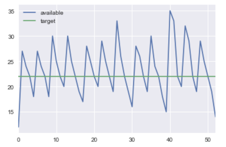
As an example, with the data above, you can compute the purchase amounts. In this case let’s assume the incoming_availability is 12 and our target is twice the biggest week’s usage: 22, it looks like this:

purchase: 19
current available: 31
current available: 27
current available: 24
current available: 22
purchase: 12
current available: 30
current available: 27
current available: 24
current available: 22
purchase: 15
current available: 33
current available: 30
current available: 25
current available: 22
purchase: 14
current available: 34
current available: 30
current available: 25
current available: 22
current available: 19
purchase: 15
current available: 32
current available: 28
current available: 25
current available: 22
purchase: 15
current available: 35
current available: 29
current available: 25
current available: 22
purchase: 16
current available: 35
current available: 33
current available: 26
current available: 22
current available: 19
purchase: 16
current available: 32
current available: 28
current available: 26
current available: 22
purchase: 14
current available: 33
current available: 30
current available: 24
current available: 22
current available: 18
purchase: 23
current available: 38
current available: 35
current available: 33
current available: 22
purchase: 16
current available: 36
current available: 32
current available: 29
current available: 22
purchase: 12
current available: 31
current available: 29
current available: 25
current available: 22
current available: 19